Implementation Details

RfbFoam builds upon the Lattice Optimization for Porous Electrodes (LOPE) model by Beck et al. The original codebase has been substantially transformed into a generalized, validated half-cell model for simulating transport phenomena in redox flow batteries.

Key Modifications from LOPE

The most significant changes implemented to increase the physical relevance include:

• Removing the optimization-relevant quantities while keeping porosity-dependent properties
• Decoupling the physical properties from the pore-scale dataset, enabling independent setting of $\varepsilon$, $a$, $k_{\text{m,O}}$, $k_{\text{m,R}}$ and $K$
• Altering the momentum equation to be consistent with the volume-averaged velocity $\vec{v}$
• Modifying the expression for $i_{\text{loc}}$ to be consistent for cases where $C_{\text{ref}} \neq 1$
• Adding Nernst correction to the standard potential
• Adding the Forchheimer coefficient $\beta$ to the momentum equation
• Adding an optional alternative definition for effective properties based on tortuosity rather than the Bruggeman correlation
• Changing the membrane boundary condition to a potentiostatic condition

Additional features:

• Generalizing RFB geometry definition for complex and realistic cell configurations
• Decomposing the cell overpotential into electrolyte/electrode ohmic losses and kinetic/transport losses
• Extending the logging system (flow rates, species rates, concentrations, SoC, pressure drop, current density, overpotential)
• Support for defining gradients in physical and microstructural properties (e.g., porosity gradient) — see Spatially-Variable Fields
• Modular code structure for easier maintenance and extensibility

Solution Algorithm

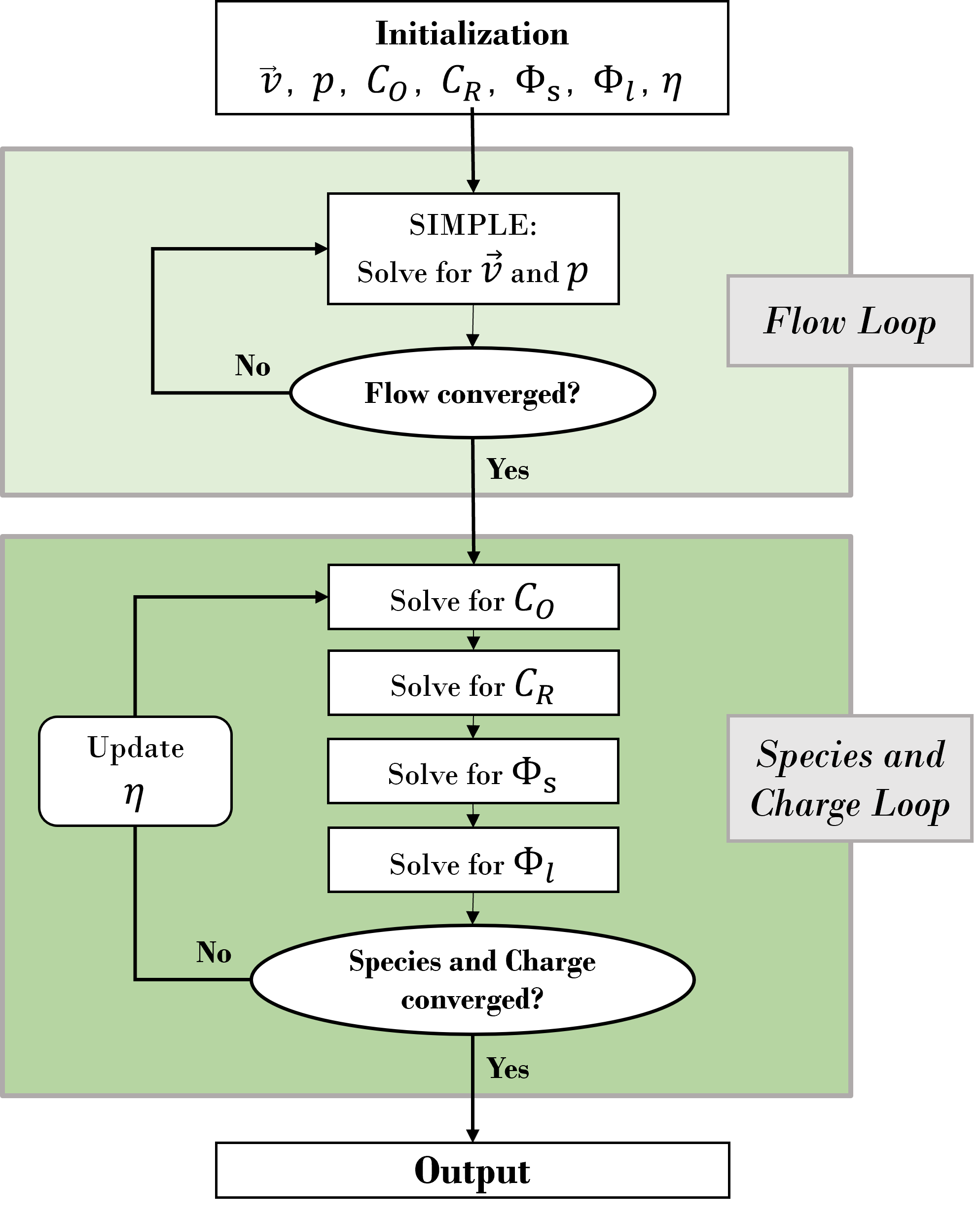
Schematic diagram of the steady-state solution algorithm used by RfbFoam.

The algorithm proceeds as follows:

1. Initialization of field variables
2. Flow loop: Iteratively solve momentum and continuity equations using SIMPLE until the sum of residuals for $\vec{v}$ and $p$ reaches below $10^{-5}$
3. Species and charge loop: Once flow is converged, solve concentration and potential fields until residuals for $C_{\text{O}}$, $C_{\text{R}}$, $\Phi_{\text{s}}$, and $\Phi_{\text{l}}$ reach below $10^{-5}$
4. After each iteration, update $\eta$ according to the newly calculated potential and concentration fields

tip

The flow loop can be performed independently from the species/charge loop. This is useful for making polarization curves since the velocity field remains fixed — run the flow once and reuse results across different applied potentials. Use the -onlyU and -onlyScalar flags for this (see Solver Options).

Bruggeman Correlation vs. Tortuosity

While most RFB models rely on the Bruggeman correlation, RfbFoam primarily utilizes explicit porosity and tortuosity parameters. The effective diffusion coefficient is calculated as:

$$D_i^{\text{eff}} = D_i \cdot \frac{\varepsilon}{\tau}$$

where $\tau$ is the tortuosity factor measured directly from experiments. The electronic conductivity $\kappa^{\text{eff}}$ is set as a direct input field, and the ionic conductivity $\sigma^{\text{eff}}$ is defined as a constant.

note

Users can revert to the Bruggeman correlation through simple modifications in the source code if desired.