Case Setup

This page describes how RfbFoam cases are structured and how to configure the geometry, mesh, and physical properties for your simulations.

Case Directory Structure

Each RfbFoam case follows the standard OpenFOAM directory layout:

<case>/
├── Allrun                  # Run script
├── Allclean                # Clean script
├── 0/                      # Initial and boundary conditions
│   ├── U, p                # Flow fields
│   ├── CO, CR              # Species concentration fields
│   ├── Phi1, Phi2          # Potential fields
│   └── porosity, kappa1, … # Material property fields
├── 0.orig/                 # Original fields overwritten by setExprFields
│   ├── areaPerVol          # Specific surface area
│   ├── invPermeability     # Inverse permeability
│   ├── kappa1              # Solid-phase conductivity
│   ├── porosity            # Electrode porosity
│   └── tau                 # Tortuosity
├── constant/
│   ├── transportProperties # Physical and electrochemical parameters
│   ├── turbulenceProperties
│   └── triSurface/         # STL geometry files
└── system/
    ├── controlDict         # Simulation control
    ├── fvSchemes           # Discretization schemes
    ├── fvSolution          # Linear solver settings
    ├── blockMeshDict       # Background mesh definition
    ├── snappyHexMeshDict   # Mesh refinement
    └── decomposeParDict    # Parallel decomposition settings

Field Variables

RfbFoam defines two sets of OpenFOAM fields:

Category	Fields
Solved variables	$\vec{v}$, $p$, $C_{\text{O}}$, $C_{\text{R}}$, $\Phi_{\text{s}}$, $\Phi_{\text{l}}$
Physical properties	$\varepsilon$, $a$, $k_{\text{m,O}}$, $k_{\text{m,R}}$, $K$, $\tau$

Each physical property can be set independently or as a function of others (e.g., porosity). The properties in flow channels are configured for non-reactive free flow: $\varepsilon = 0.99$, $a = 0$, and $K^{-1} = \beta = 0$. This is handled by the OpenFOAM built-in tool setExprFields. For details on configuring uniform or spatially-varying properties (e.g., porosity gradients), see Spatially-Variable Fields.

Cell Configurations

RfbFoam supports different electrode-flow field configurations. Two configurations are provided as examples:

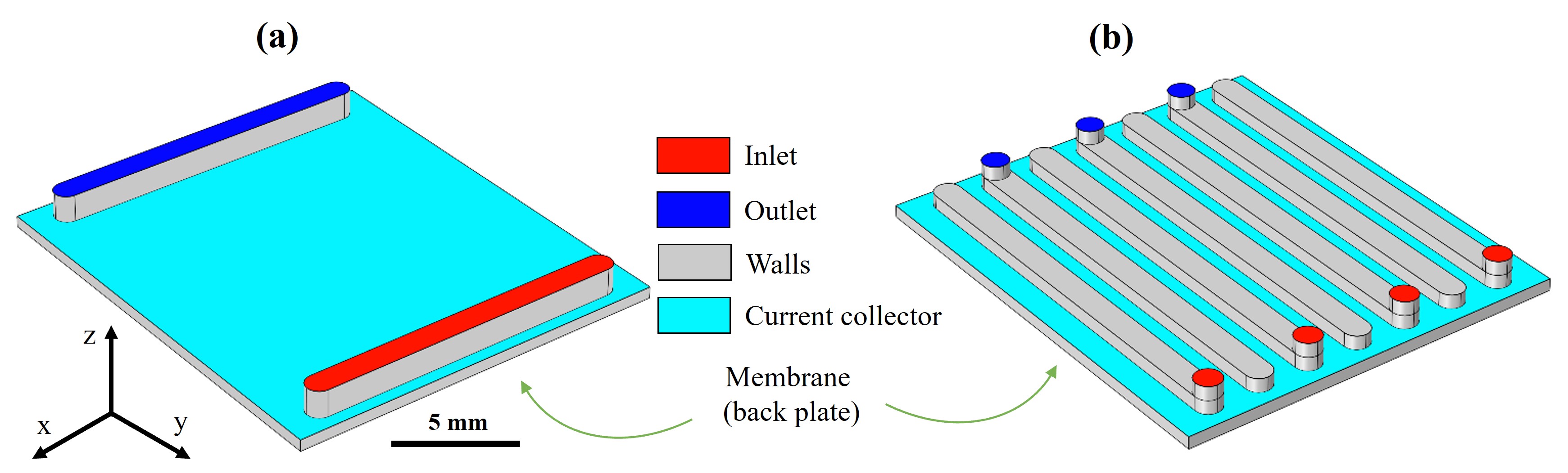Schematic of the 3D FTFF (a) and IDFF (b) electrode-flow field geometries. The computational domains are composed of the porous electrode and flow channels. Red and blue surfaces indicate inlet and outlet. Gray and cyan show the current collector and walls. The membrane is the back plate.

Boundary Types

Five types of boundaries are distinguished:

Boundary	Physical meaning
$\Gamma_{\text{inlet}}$	Surfaces through which fluid enters
$\Gamma_{\text{outlet}}$	Surfaces through which fluid exits
$\Gamma_{\text{mem}}$	Electrode-membrane interface
$\Gamma_{\text{cc}}$	Bipolar plate (current collector) surface
$\Gamma_{\text{walls}}$	Non-conductive surfaces (gaskets, etc.)

Geometrical Parameters

The electrode dimensions used in the provided examples:

• Thickness $t_{\text{e}}$ (z-direction): 470 µm
• Length $l_{\text{e}}$ (y-direction): 17 mm
• Width $w_{\text{e}}$ (x-direction): 15 mm
• Channel depth and width: 1.0 mm

Geometry	Channel length $l_{\text{ch}}$ [mm]	Rib width [mm]	No. of channels $N_{\text{c}}$	Superficial velocity $v_{\text{e}}$
FTFF	13	14	2	$v_{\text{e}} = Q/(t_{\text{e}} \cdot w_{\text{e}})$
IDFF	16	1	7	$v_{\text{e}} = Q/((N-1) \cdot l_{\text{ch}} \cdot t_{\text{e}})$

Mesh Generation

OpenFOAM's built-in snappyHexMesh utility generates a hexahedral mesh within surfaces provided by external STL files. The input STL files are separate for each boundary type and placed in the constant/triSurface/ directory.

Using the castellatedMesh mode, snappyHexMesh trims a background mesh (defined by blockMesh) to match the geometry's enclosed volume.

Mesh refinement can be controlled to add refined cells on surfaces, especially on $\Gamma_{\text{mem}}$ and $\Gamma_{\text{cc}}$, to properly resolve gradients near edges and bounding surfaces.

Case	Mesh cells
FTFF	454K
IDFF	677K

tip

To define your own geometry, prepare STL files for each boundary type (inlet, outlet, membrane, current collector, walls) and place them in constant/triSurface/. Then update snappyHexMeshDict to reference your STL files and set appropriate refinement levels.